User Manual

Author

Liangliang Nan

Introduction

This package implements a hypothesis-and-selection based method for piecewise planar object reconstruction from point clouds [1]. The method takes as input an unordered point set sampled from a piecewise planar object. The output is a compact and watertight surface mesh interpolating the input point set. The method assumes that all necessary major planes are provided (or can be extracted from the input point set using the shape detection method described in Shape Detection, or any other alternative methods).

The existing surface reconstruction methods available in CGAL (i.e., Poisson Surface Reconstruction, Advancing Front Surface Reconstruction, and Scale-Space Surface Reconstruction) are suitable for point set representing objects described by smooth surfaces. For man-made objects such as buildings, the results are not satisfactory due to the imperfections and complexity of the reconstructed models (i.e., gigantic meshes, missing regions, noises, and undesired structures). This is mainly because these methods tend to closely follow the surface details. The algorithm introduced in this package is intended to produce simplified and watertight surface meshes. It can recover sharp features of the objects, and it can handle a large amount of noise and outliers, complementing other surface reconstruction methods.

A mixed integer programming (MIP) solver is required to solve the constrained optimization problem formulated by the method (see CGAL and Solvers).

Algorithm

Unlike traditional piecewise planar object reconstruction methods that focus on either extracting good geometric primitives or obtaining proper arrangements of primitives, the emphasis of this method lies in intersecting the primitives (i.e. planes) and seeking for an appropriate combination of them to obtain a manifold and watertight polygonal surface model.

The method casts surface reconstruction as a binary labeling problem based on a hypothesizing-and-selection strategy. The reconstruction consists in the following steps:

1. extract planes from the input point set (can be skipped if planes are known or provided by other means);
2. generate a set of candidate faces by intersecting the extracted planar primitives;
3. select an optimal subset of the candidate faces through optimization under hard constraints that enforces the final polygonal surface to be topologically correct.

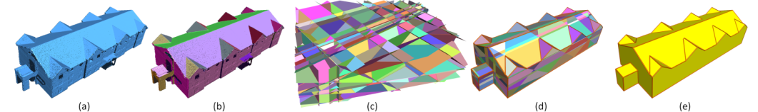
Figure 72.1 Polygonal surface reconstruction

(a) Input point set; (b) Extracted planar segments; (c) Candidate faces generated by pairwise intersection; (d) Faces selected through optimization; (e) Reconstructed model.

Energy Terms

Given \( N \) candidate faces \(F = \{f_i | 1 \leq i \leq N\}\) generated by pairwise intersection, the optimal subset of the candidate faces that best describes the geometry of the object and form a manifold and watertight polygonal surface is selected through optimization.

Let \(X = \{x_i | 1 \leq i \leq N\}\) denote the selection of the faces (i.e., \(f_i\) is chosen if \(x_i = 1\) or not chosen if \(x_i = 0\)), the objective function consists of three energy terms: data-fitting, model complexity, and point coverage.

• Data-fitting. This term is intended to evaluate the fitting quality of the faces to the point cloud. It is defined to measure a confidence-weighted percentage of points that do not contribute to the final reconstruction.

  \begin{equation} E_f = 1 - \frac{1}{|P|} \sum_{i=1}^N x_i \cdot support(f_i), \label{eq:datafitting} \end{equation}

  \(|P|\) is the total number of points in \(P\). \(support(f_i)\) is the number of supporting points accounting for an appropriate notion of confidence.

• Model complexity. This term is to encourage simple structures (i.e., large planar regions). It is defined as the ratio of sharp edges in the model.

  \begin{equation} E_m = \frac{1}{|E|}\sum_{i=1}^{|E|} corner(e_i), \label{eq:complexity} \end{equation}

  \(|E|\) denotes the total number of pairwise intersections in the candidate face set. \(corner(e_i)\) is an indicator function whose value is determined by the configuration of the two selected faces connected by \(e_i\). \(corner(e_i)\) will have a value of 1 if the faces associated with \(e_i\) introduce a sharp edge in the final model. Otherwise, \(corner(e_i)\) has a zero value meaning the two faces are coplanar.

• Point coverage. This term is intended to handle missing data. The idea is to keep the unsupported regions (i.e., regions not covered by points) of the final model as small as possible. This term is defined as the ratio of uncovered regions in the model.

  \begin{equation} E_c = \frac{1}{area(M)}\sum_{i=1}^N x_i \cdot (area(f_i) - area(M_i^\alpha)), \label{eq:coverage} \end{equation}

  Here \(area(M)\), \(area(f_i)\), and \(area(M_i^\alpha)\) denote the surface areas of the final model, a candidate face \(f_i\), and the \(\alpha\)-shape mesh \(M_i^\alpha\) of \(f_i\), respectively. The \(area(M_i^\alpha)\) is to approximate the area of the face covered by the 3D points.

  For more details on the energy terms and the formulation, please refer to the original paper [1].

Face Selection

With the above energy terms, the optimal set of faces can be obtained by minimizing a weighted sum of these terms under certain hard constraints.

\begin{equation} \begin{aligned} \underset{\mathbf{X}}{\text{min}} \quad & \lambda_f \cdot E_f + \lambda_m \cdot E_m + \lambda_c \cdot E_c \\ \text{s.t.} \quad & \begin{cases} \begin{aligned} & \sum_{j \in \mathcal{N}(e_i)} {x_j} = 2 \quad \text{or} \quad 0, && 1 \leq i \leq |E| \\ & x_i \in \{0, 1\}, && 1 \leq i \leq N \end{aligned} \end{cases} \end{aligned} \label{eq:optimization} \end{equation}

Here \( \sum_{j \in \mathcal{N}(e_i)} {x_j} \) counts the number of faces connected by an edge \( e_i \). This value is enforced to be either 0 or 2, meaning none or two of the faces can be selected. These hard constraints guarantee that each edge of the final model connects only two adjacent faces.

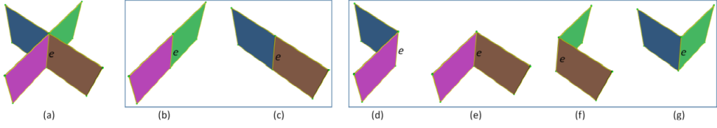
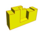
Figure 72.2 Intersection of two planes

Two planes intersect with each other resulting in four parts (a). (b) to (g) show all possible combinations to ensure a 2-manifold surface. The edge in (b) and (c) connects two co-planar parts, while in (d) to (g) it introduces sharp edges in the final model.

Examples

Reconstruction from Point Clouds

The method assumes that all necessary planes can be extracted from the input point set. The following examples first extract planes from the input point cloud and then reconstruct the surface model. In the first example, the Efficient RANSAC approach is used to extract planes. It is very fast, but not deterministic, as opposed to the region growing approach from the second example that is slower, but more precise and always returns the same result for the same given parameters.

Example: Polygonal_surface_reconstruction/polyfit_example_without_input_planes.cpp

Show / Hide

#include <CGAL/Exact_predicates_inexact_constructions_kernel.h>
#include <CGAL/IO/read_points.h>
#include <CGAL/property_map.h>
#include <CGAL/Surface_mesh.h>
#include <CGAL/Shape_detection/Efficient_RANSAC.h>
#include <CGAL/Polygonal_surface_reconstruction.h>
 
#ifdef CGAL_USE_SCIP  // defined (or not) by CMake scripts, do not define by hand
 
#include <CGAL/SCIP_mixed_integer_program_traits.h>
typedef CGAL::SCIP_mixed_integer_program_traits<double>                        MIP_Solver;
 
#elif defined(CGAL_USE_GLPK)  // defined (or not) by CMake scripts, do not define by hand
 
#include <CGAL/GLPK_mixed_integer_program_traits.h>
typedef CGAL::GLPK_mixed_integer_program_traits<double>                        MIP_Solver;
 
#endif
 
 
#if defined(CGAL_USE_GLPK) || defined(CGAL_USE_SCIP)
 
#include <CGAL/Timer.h>
 
#include <fstream>
 
 
typedef CGAL::Exact_predicates_inexact_constructions_kernel                        Kernel;
 
typedef Kernel::Point_3                                                                                                Point;
typedef Kernel::Vector_3                                                                                        Vector;
 
// Point with normal, and plane index
typedef boost::tuple<Point, Vector, int>                                                        PNI;
typedef std::vector<PNI>                                                                                        Point_vector;
typedef CGAL::Nth_of_tuple_property_map<0, PNI>                                                Point_map;
typedef CGAL::Nth_of_tuple_property_map<1, PNI>                                                Normal_map;
typedef CGAL::Nth_of_tuple_property_map<2, PNI>                                                Plane_index_map;
 
typedef CGAL::Shape_detection::Efficient_RANSAC_traits<Kernel, Point_vector, Point_map, Normal_map>     Traits;
 
typedef CGAL::Shape_detection::Efficient_RANSAC<Traits>             Efficient_ransac;
typedef CGAL::Shape_detection::Plane<Traits>                                                Plane;
typedef CGAL::Shape_detection::Point_to_shape_index_map<Traits>     Point_to_shape_index_map;
 
typedef        CGAL::Polygonal_surface_reconstruction<Kernel>                                Polygonal_surface_reconstruction;
typedef CGAL::Surface_mesh<Point>                                                                        Surface_mesh;
 
/*
* This example first extracts planes from the input point cloud
* (using RANSAC with default parameters) and then reconstructs
* the surface model from the planes.
*/
 
int main(int argc, char* argv[])
{
  Point_vector points;
 
  // Loads point set from a file.
  const std::string input_file = (argc > 1) ? argv[1] : CGAL::data_file_path("points_3/cube.pwn");
  std::ifstream input_stream(input_file.c_str());
  if (input_stream.fail()) {
    std::cerr << "failed open file \'" <<input_file << "\'" << std::endl;
    return EXIT_FAILURE;
  }
  input_stream.close();
  std::cout << "Loading point cloud: " << input_file << "...";
 
  CGAL::Timer t;
  t.start();
  if (!CGAL::IO::read_points(input_file.c_str(), std::back_inserter(points),
                             CGAL::parameters::point_map(Point_map()).normal_map(Normal_map())))
  {
    std::cerr << "Error: cannot read file " << input_file << std::endl;
    return EXIT_FAILURE;
  }
  else
    std::cout << " Done. " << points.size() << " points. Time: " << t.time() << " sec." << std::endl;
 
  // Shape detection
  Efficient_ransac ransac;
  ransac.set_input(points);
  ransac.add_shape_factory<Plane>();
 
  std::cout << "Extracting planes...";
  t.reset();
  ransac.detect();
 
  Efficient_ransac::Plane_range planes = ransac.planes();
  std::size_t num_planes = planes.size();
 
  std::cout << " Done. " << num_planes << " planes extracted. Time: " << t.time() << " sec." << std::endl;
 
  // Stores the plane index of each point as the third element of the tuple.
  Point_to_shape_index_map shape_index_map(points, planes);
  for (std::size_t i = 0; i < points.size(); ++i) {
    // Uses the get function from the property map that accesses the 3rd element of the tuple.
    int plane_index = get(shape_index_map, i);
    points[i].get<2>() = plane_index;
  }

 
  std::cout << "Generating candidate faces...";
  t.reset();
 
  Polygonal_surface_reconstruction algo(
    points,
    Point_map(),
    Normal_map(),
    Plane_index_map()
  );
 
  std::cout << " Done. Time: " << t.time() << " sec." << std::endl;

 
  Surface_mesh model;
 
  std::cout << "Reconstructing...";
  t.reset();
 
  if (!algo.reconstruct<MIP_Solver>(model)) {
    std::cerr << " Failed: " << algo.error_message() << std::endl;
    return EXIT_FAILURE;
  }
 
  const std::string& output_file("without_input_planes_result.off");
  if (CGAL::IO::write_OFF(output_file, model))
    std::cout << " Done. Saved to " << output_file << ". Time: " << t.time() << " sec." << std::endl;
  else {
    std::cerr << " Failed saving file." << std::endl;
    return EXIT_FAILURE;
  }

 
  // Also stores the candidate faces as a surface mesh to a file
  Surface_mesh candidate_faces;
  algo.output_candidate_faces(candidate_faces);
  const std::string& candidate_faces_file("without_input_planes_cube_candidate_faces.off");
  std::ofstream candidate_stream(candidate_faces_file.c_str());
  if (CGAL::IO::write_OFF(candidate_stream, candidate_faces))
    std::cout << "Candidate faces saved to " << candidate_faces_file << "." << std::endl;
 
  return EXIT_SUCCESS;
}
 
 
#else
 
int main(int, char**)
{
    std::cerr << "This test requires either GLPK or SCIP.\n";
    return EXIT_SUCCESS;
}
 
#endif  // defined(CGAL_USE_GLPK) || defined(CGAL_USE_SCIP)

Example: Polygonal_surface_reconstruction/polyfit_example_with_region_growing.cpp

Show / Hide

#include <CGAL/Exact_predicates_inexact_constructions_kernel.h>
#include <CGAL/IO/read_points.h>
#include <CGAL/property_map.h>
#include <CGAL/Surface_mesh.h>
#include <CGAL/Shape_detection/Region_growing/Region_growing.h>
#include <CGAL/Shape_detection/Region_growing/Point_set.h>
#include <CGAL/Polygonal_surface_reconstruction.h>
 
#ifdef CGAL_USE_SCIP  // defined (or not) by CMake scripts, do not define by hand
 
#include <CGAL/SCIP_mixed_integer_program_traits.h>
typedef CGAL::SCIP_mixed_integer_program_traits<double> MIP_Solver;
 
#elif defined(CGAL_USE_GLPK)  // defined (or not) by CMake scripts, do not define by hand
 
#include <CGAL/GLPK_mixed_integer_program_traits.h>
typedef CGAL::GLPK_mixed_integer_program_traits<double>        MIP_Solver;
 
#endif
 
#if defined(CGAL_USE_GLPK) || defined(CGAL_USE_SCIP)
 
#include <fstream>
#include <CGAL/Timer.h>
#include <boost/range/irange.hpp>
 
typedef CGAL::Exact_predicates_inexact_constructions_kernel        Kernel;
 
typedef Kernel::FT       FT;
typedef Kernel::Point_3         Point;
typedef Kernel::Vector_3 Vector;
 
// Point with normal, and plane index.
typedef boost::tuple<Point, Vector, int> PNI;
typedef std::vector<PNI> Point_vector;
 
typedef CGAL::Nth_of_tuple_property_map<0, PNI>        Point_map;
typedef CGAL::Nth_of_tuple_property_map<1, PNI>        Normal_map;
typedef CGAL::Nth_of_tuple_property_map<2, PNI>        Plane_index_map;
 
using Point_map_region_growing = CGAL::Compose_property_map<CGAL::Random_access_property_map<Point_vector>, Point_map >;
using Normal_map_region_growing = CGAL::Compose_property_map<CGAL::Random_access_property_map<Point_vector>, Normal_map >;
 
using Region_type = CGAL::Shape_detection::Point_set::Least_squares_plane_fit_region<Kernel, std::size_t, Point_map_region_growing, Normal_map_region_growing>;
using Neighbor_query = CGAL::Shape_detection::Point_set::Sphere_neighbor_query<Kernel, std::size_t, Point_map_region_growing>;
using Region_growing = CGAL::Shape_detection::Region_growing<Neighbor_query, Region_type>;
 
typedef CGAL::Surface_mesh<Point>        Surface_mesh;
typedef CGAL::Polygonal_surface_reconstruction<Kernel> Polygonal_surface_reconstruction;
 
/*
* This example first extracts planes from the input point cloud
* (using region growing) and then reconstructs
* the surface model from the planes.
*/
 
int main(int argc, char* argv[])
{
  Point_vector points;
 
  // Load point set from a file.
  const std::string input_file = (argc > 1) ? argv[1] : CGAL::data_file_path("points_3/cube.pwn");
  std::ifstream input_stream(input_file.c_str());
  if (input_stream.fail()) {
    std::cerr << "Failed open file \'" << input_file << "\'" << std::endl;
    return EXIT_FAILURE;
  }
  input_stream.close();
  std::cout << "Loading point cloud: " << input_file << "...";
 
  CGAL::Timer t;
  t.start();
  if (!CGAL::IO::read_points(input_file.c_str(), std::back_inserter(points),
    CGAL::parameters::point_map(Point_map()).normal_map(Normal_map()))) {
 
    std::cerr << "Error: cannot read file " << input_file << std::endl;
    return EXIT_FAILURE;
  }
  else
    std::cout << " Done. " << points.size() << " points. Time: "
    << t.time() << " sec." << std::endl;

 
  // Shape detection.
 
  // Default parameter values for the data file cube.pwn.
  const FT          search_sphere_radius = FT(2) / FT(100);
  const FT          max_distance_to_plane = FT(2) / FT(1000);
  const FT          max_accepted_angle = FT(25);
  const std::size_t min_region_size = 200;
 
  Point_map_region_growing point_map_rg(CGAL::make_random_access_property_map(points));
  Normal_map_region_growing normal_map_rg(CGAL::make_random_access_property_map(points));
 
  // Create instances of the classes Neighbor_query and Region_type.
  Neighbor_query neighbor_query(
    boost::irange<std::size_t>(0, points.size()), CGAL::parameters::sphere_radius(search_sphere_radius).point_map(point_map_rg));
 
  Region_type region_type(
    CGAL::parameters::
    maximum_distance(max_distance_to_plane).
    maximum_angle(max_accepted_angle).
    minimum_region_size(min_region_size).
    point_map(point_map_rg).
    normal_map(normal_map_rg));
 
  // Create an instance of the region growing class.
  Region_growing region_growing(
    boost::irange<std::size_t>(0, points.size()), neighbor_query, region_type);
 
  std::cout << "Extracting planes...";
  std::vector<typename Region_growing::Primitive_and_region> regions;
  t.reset();
  region_growing.detect(std::back_inserter(regions));
  std::cout << " Done. " << regions.size() << " planes extracted. Time: "
    << t.time() << " sec." << std::endl;
 
  // Stores the plane index of each point as the third element of the tuple.
  for (std::size_t i = 0; i < points.size(); ++i)
    // Uses the get function from the property map that accesses the 3rd element of the tuple.
    points[i].get<2>() = static_cast<int>(get(region_growing.region_map(), i));

 
  // Reconstruction.
 
  std::cout << "Generating candidate faces...";
  t.reset();
  Polygonal_surface_reconstruction algo(
    points,
    Point_map(),
    Normal_map(),
    Plane_index_map()
  );
  std::cout << " Done. Time: " << t.time() << " sec." << std::endl;
 
  Surface_mesh model;
  std::cout << "Reconstructing...";
  t.reset();
  if (!algo.reconstruct<MIP_Solver>(model)) {
    std::cerr << "Failed: " << algo.error_message() << std::endl;
    return EXIT_FAILURE;
  }
  std::cout << " Done. Time: " << t.time() << " sec." << std::endl;
 
  std::cout << "Saving...";
  t.reset();
  const std::string& output_file("with_region_growing_result.off");
  if (CGAL::IO::write_OFF(output_file, model))
    std::cout << " Done. Saved to " << output_file << ". Time: " << t.time() << " sec." << std::endl;
  else {
    std::cerr << " Failed saving file." << std::endl;
    return EXIT_FAILURE;
  }
 
  return EXIT_SUCCESS;
}
 
#else
 
int main(int, char**)
{
  std::cerr << "This test requires either GLPK or SCIP.\n";
  return EXIT_SUCCESS;
}
 
#endif  // defined(CGAL_USE_GLPK) || defined(CGAL_USE_SCIP)

Reconstruction with User-Provided Planes

The following example shows the reconstruction using user-provided planar segments.

Example: Polygonal_surface_reconstruction/polyfit_example_user_provided_planes.cpp

Show / Hide

#include <CGAL/Exact_predicates_inexact_constructions_kernel.h>
#include <CGAL/IO/read_points.h>
#include <CGAL/property_map.h>
#include <CGAL/Surface_mesh.h>
#include <CGAL/Polygonal_surface_reconstruction.h>
 
#ifdef CGAL_USE_SCIP  // defined (or not) by CMake scripts, do not define by hand
#include <CGAL/SCIP_mixed_integer_program_traits.h>
typedef CGAL::SCIP_mixed_integer_program_traits<double>                        MIP_Solver;
#elif defined(CGAL_USE_GLPK)  // defined (or not) by CMake scripts, do not define by hand
#include <CGAL/GLPK_mixed_integer_program_traits.h>
typedef CGAL::GLPK_mixed_integer_program_traits<double>                        MIP_Solver;
#endif
 
 
#if defined(CGAL_USE_GLPK) || defined(CGAL_USE_SCIP)
 
#include <CGAL/Timer.h>
 
#include <fstream>
 
 
typedef CGAL::Exact_predicates_inexact_constructions_kernel                Kernel;
typedef Kernel::Point_3                                                                                        Point;
typedef Kernel::Vector_3                                                                                Vector;
typedef        CGAL::Polygonal_surface_reconstruction<Kernel>                        Polygonal_surface_reconstruction;
typedef CGAL::Surface_mesh<Point>                                                                Surface_mesh;
 
// Point with normal, and plane index
typedef boost::tuple<Point, Vector, int>                                                PNI;
typedef CGAL::Nth_of_tuple_property_map<0, PNI>                                        Point_map;
typedef CGAL::Nth_of_tuple_property_map<1, PNI>                                        Normal_map;
typedef CGAL::Nth_of_tuple_property_map<2, PNI>                                        Plane_index_map;
 
/*
* The following example shows the reconstruction using user-provided
* planar segments stored in PLY format. In the PLY format, a property
* named "segment_index" stores the plane index for each point (-1 if
* the point is not assigned to a plane).
*/
 
int main(int argc, char* argv[])
{
  const std::string input_file = (argc > 1) ? argv[1] : CGAL::data_file_path("points_3/ball.ply");
  std::ifstream input_stream(input_file.c_str());
 
  std::vector<PNI> points; // store points
 
  std::cout << "Loading point cloud: " << input_file << "...";
  CGAL::Timer t;
  t.start();
 
  if (!CGAL::IO::read_PLY_with_properties(input_stream,
                                          std::back_inserter(points),
                                          CGAL::IO::make_ply_point_reader(Point_map()),
                                          CGAL::IO::make_ply_normal_reader(Normal_map()),
                                          std::make_pair(Plane_index_map(), CGAL::IO::PLY_property<int>("segment_index"))))
  {
    std::cerr << "Error: cannot read file " << input_file << std::endl;
    return EXIT_FAILURE;
  }
  else
    std::cout << " Done. " << points.size() << " points. Time: " << t.time() << " sec." << std::endl;

 
  std::cout << "Generating candidate faces...";
  t.reset();
 
  Polygonal_surface_reconstruction algo(
    points,
    Point_map(),
    Normal_map(),
    Plane_index_map()
  );
 
  std::cout << " Done. Time: " << t.time() << " sec." << std::endl;

 
  Surface_mesh model;
 
  std::cout << "Reconstructing...";
  t.reset();
 
  if (!algo.reconstruct<MIP_Solver>(model)) {
    std::cerr << " Failed: " << algo.error_message() << std::endl;
    return EXIT_FAILURE;
  }
 
  // Saves the mesh model
    const std::string& output_file("user_provided_planes_result.off");
    if (CGAL::IO::write_OFF(output_file, model))
        std::cout << " Done. Saved to " << output_file << ". Time: " << t.time() << " sec." << std::endl;
    else {
        std::cerr << " Failed saving file." << std::endl;
        return EXIT_FAILURE;
    }
 
  return EXIT_SUCCESS;
}
 
 
#else
 
int main(int, char**)
{
    std::cerr << "This test requires either GLPK or SCIP.\n";
    return EXIT_SUCCESS;
}
 
#endif  // defined(CGAL_USE_GLPK) || defined(CGAL_USE_SCIP)

Model Complexity Control

In addition to favoring clean and compact reconstruction results by encouraging large planar regions, the model complexity term also provides control over the model details, i.e., increasing the influence of this term results in fewer details in the reconstructed 3D models.

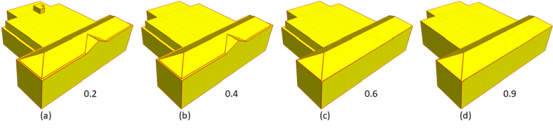
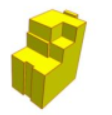
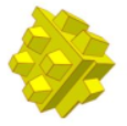
Figure 72.3 The effect of the model complexity term

Reconstruction by gradually increasing the influence of the model complexity term. The values under each subfigure are the weights used in the corresponding optimization.

The following example shows how to control the model complexity by tuning the weight of the model complexity term.

Remarks

This example also shows how to reuse the intermediate results from the candidate generation step.

Example: Polygonal_surface_reconstruction/polyfit_example_model_complexity_control.cpp

Show / Hide

#include <CGAL/Exact_predicates_inexact_constructions_kernel.h>
#include <CGAL/IO/read_points.h>
#include <CGAL/property_map.h>
#include <CGAL/Surface_mesh.h>
#include <CGAL/Polygonal_surface_reconstruction.h>
 
#ifdef CGAL_USE_SCIP // defined (or not) by CMake scripts, do not define by hand
#include <CGAL/SCIP_mixed_integer_program_traits.h>
typedef CGAL::SCIP_mixed_integer_program_traits<double>                        MIP_Solver;
#elif defined(CGAL_USE_GLPK) // defined (or not) by CMake scripts, do not define by hand
#include <CGAL/GLPK_mixed_integer_program_traits.h>
typedef CGAL::GLPK_mixed_integer_program_traits<double>                        MIP_Solver;
#endif
 
 
#if defined(CGAL_USE_GLPK) || defined(CGAL_USE_SCIP)
 
#include <CGAL/Timer.h>
 
#include <fstream>
 
 
typedef CGAL::Exact_predicates_inexact_constructions_kernel                Kernel;
typedef Kernel::Point_3                                                                                        Point;
typedef Kernel::Vector_3                                                                                Vector;
typedef        CGAL::Polygonal_surface_reconstruction<Kernel>                        Polygonal_surface_reconstruction;
typedef CGAL::Surface_mesh<Point>                                                                Surface_mesh;
 
// Point with normal, and plane index
typedef boost::tuple<Point, Vector, int>                                                PNI;
typedef CGAL::Nth_of_tuple_property_map<0, PNI>                                        Point_map;
typedef CGAL::Nth_of_tuple_property_map<1, PNI>                                        Normal_map;
typedef CGAL::Nth_of_tuple_property_map<2, PNI>                                        Plane_index_map;
 
/*
* The following example shows how to control the model complexity by
* increasing the influence of the model complexity term.
* In this example, the intermediate results from plane extraction and
* candidate generation are cached and reused.
*/
 
int main(int argc, char* argv[])
{
  const std::string input_file = (argc > 1) ? argv[1] : CGAL::data_file_path("points_3/building.ply");
  std::ifstream input_stream(input_file.c_str());
 
  std::vector<PNI> points; // store points
 
  std::cout << "Loading point cloud: " << input_file << "...";
  CGAL::Timer t;
  t.start();
 
  if (!CGAL::IO::read_PLY_with_properties(input_stream,
                                          std::back_inserter(points),
                                          CGAL::IO::make_ply_point_reader(Point_map()),
                                          CGAL::IO::make_ply_normal_reader(Normal_map()),
                                          std::make_pair(Plane_index_map(), CGAL::IO::PLY_property<int>("segment_index"))))
  {
    std::cerr << "Error: cannot read file " << input_file << std::endl;
    return EXIT_FAILURE;
  }
  else
    std::cout << " Done. " << points.size() << " points. Time: " << t.time() << " sec." << std::endl;

 
  std::cout << "Generating candidate faces...";
  t.reset();
 
  Polygonal_surface_reconstruction algo(
    points,
    Point_map(),
    Normal_map(),
    Plane_index_map()
  );
 
  std::cout << " Done. Time: " << t.time() << " sec." << std::endl;

 
  // Reconstruction with complexity control
 
  // Model 1: more detail
  Surface_mesh model;
 
  std::cout << "Reconstructing with complexity 0.05...";
  t.reset();
  if (!algo.reconstruct<MIP_Solver>(model, 0.8, 0.15, 0.05)) {
    std::cerr << " Failed: " << algo.error_message() << std::endl;
    return EXIT_FAILURE;
  }
  else {
       const std::string& output_file = "building_result-0.05.off";
       if (CGAL::IO::write_OFF(output_file, model)) {
           std::cout << " Done. Saved to " << output_file << ". Time: " << t.time() << " sec." << std::endl;
       }
       else {
           std::cerr << " Failed saving file." << std::endl;
           return EXIT_FAILURE;
       }
  }
 
  // Model 2: a little less detail
  std::cout << "Reconstructing with complexity 0.5...";
  t.reset();
  if (!algo.reconstruct<MIP_Solver>(model, 0.3, 0.2, 0.5)) {
    std::cerr << " Failed: " << algo.error_message() << std::endl;
    return EXIT_FAILURE;
  }
  else {
       const std::string& output_file = "building_result-0.5.off";
       if (CGAL::IO::write_OFF(output_file, model))
           std::cout << " Done. Saved to " << output_file << ". Time: " << t.time() << " sec." << std::endl;
       else {
           std::cerr << " Failed saving file." << std::endl;
           return EXIT_FAILURE;
       }
  }
 
  // Model 3: more less detail
  std::cout << "Reconstructing with complexity 0.7...";
  t.reset();
  if (!algo.reconstruct<MIP_Solver>(model, 0.2, 0.1, 0.7)) {
    std::cerr << " Failed: " << algo.error_message() << std::endl;
    return EXIT_FAILURE;
  }
  else {
    const std::string& output_file = "building_result-0.7.off";
    if (CGAL::IO::write_OFF(output_file, model)){
      std::cout << " Done. Saved to " << output_file << ". Time: " << t.time() << " sec." << std::endl;
                }
    else {
      std::cerr << " Failed saving file." << std::endl;
      return EXIT_FAILURE;
    }
  }
  return EXIT_SUCCESS;
}
 
 
#else
 
int main(int, char**)
{
    std::cerr << "This test requires either GLPK or SCIP.\n";
    return EXIT_SUCCESS;
}
 
#endif  // defined(CGAL_USE_GLPK) || defined(CGAL_USE_SCIP)

Performance

The Problem Complexity

The method is intended for reconstructing single objects with reasonable geometric complexity. The current implementation computes pairwise intersections of the planar segments, which is sufficient but not necessary to ensure topologically accurate reconstructions. Running on large complex objects may result in an extremely large number of candidate faces, and thus a huge integer programming problem to be solved.

The reconstruction time of a single object with moderate complexity is typically within a few seconds. Among the three steps, the face selection step dominates the reconstruction pipeline when the number of candidate faces is large (e.g., more than 5,000).

The Numerical Solver

The current implementation incorporates two open source solvers: GLPK and SCIP (see CGAL and Solvers). It should be noted that GLPK only manages to solve small problems, i.e., objects with reasonably simple structure. In case you are reconstructing more complex objects, you may need to consider more efficient open source solvers (e.g., CBC) or even commercial solvers (e.g., Gurobi, CPLEX). The following table gives a rough idea of the performance of some solvers.

Model	Problem Size variables/constraints	Gurobi	CBC	SCIP	GLPK	LP_SOLVE
	1244/2660	0.05 sec	0.2 sec	0.3 sec	9 sec	15 min
	2582/5420	0.2 sec	0.6 sec	2.6 sec	35 min	-
	21556/442191	2 sec	7.5 sec	9 sec	-	-