Introduction
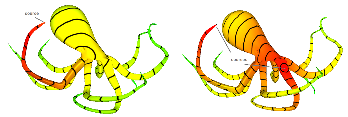
The heat method is an algorithm that solves the single- or multiple-source shortest path problem by returning an approximation of the geodesic distance for all vertices of a triangle mesh to the closest vertex in a given set of source vertices. The geodesic distance between two vertices of a mesh is the distance when walking on the surface, potentially through the interior of faces. Two vertices that are close in 3D space may be far away on the surface, for example on neighboring arms of the octopus. In the figures we color code the distance as a gradient red/green corresponding to close/far from the source vertices.
The heat method is highly efficient, since the algorithm boils down to two standard sparse linear algebra problems. It is especially useful in situations where one wishes to perform repeated distance queries on a fixed domain, since precomputation done for the first query can be reused.
As a rule of thumb, the method works well on triangle meshes, which are Delaunay, though in practice may also work fine for meshes that are far from Delaunay. In order to ensure good behavior, we enable a preprocessing step that constructs an intrinsic Delaunay triangulation (iDT); this triangulation does not change the input geometry, but generally improves the quality of the solution. The cost of this preprocessing step roughly doubles the overall preprocessing cost.
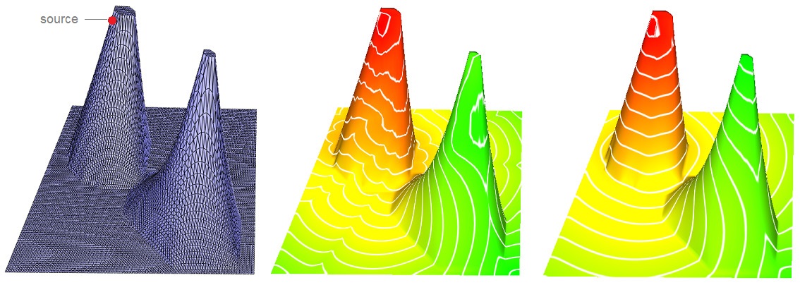
Figure 88.1 Isolines placed on a mesh without and with iDT remeshing.
In the next section we give some examples. Section Theoretical Background presents the mathematical theory of the Heat method. The last section is about the Implementation History.
Note that this package depends on the third party Eigen library (3.3 or greater), or another model of the concept SparseLinearAlgebraWithFactorTraits_d. This implementation is based on [1] , [2] , and [3]
This package is related to the package Triangulated Surface Mesh Shortest Paths. Both deal with geodesic distances. The heat method package computes for every vertex of a mesh an approximate distance to one or several source vertices. The geodesic shortest path package computes the exact shortest path between any two points on the surface.
Examples
We give examples for the free function CGAL::Heat_method_3::estimate_geodesic_distances(), for the class template CGAL::Heat_method_3::Surface_mesh_geodesic_distances_3, with and without the use of intrinsic Delaunay triangulation.
Using a Free Function
The first example calls the free function Heat_method_3::estimate_geodesic_distances(), which computes for all vertices of a triangle mesh the distances to a single source vertex.
The distances are written into an internal property map of the surface mesh.
Example: Heat_method_3/heat_method.cpp
Show / Hide
For a Polyhedron_3 you can either add a data field to the vertex type, or, as shown in the following example, create a boost::unordered_map and pass it to the function boost::make_assoc_property_map(), which generates a vertex distance property map.
Example: Heat_method_3/heat_method_polyhedron.cpp
Show / Hide
Using the Heat Method Class
The following example shows the heat method class. It can be used when one adds and removes source vertices. It performs a precomputation, which depend only on the input mesh and not the particular set of source vertices. In the example we compute the distances to one source, add the farthest vertex as a second source vertex, and then compute the distances with respect to these two sources.
Example: Heat_method_3/heat_method_surface_mesh.cpp
Show / Hide
Switching off the Intrinsic Delaunay Triangulation
The following example shows the heat method on a triangle mesh without using the intrinsic Delaunay triangulation (iDT) algorithm, for example because by construction your meshes have a good quality (Poor quality in this case means that the input is far from Delaunay, though even in this case one may still get good results without iDT, depending on the specific geometry of the surface). The iDT algorithm is switched off by the template parameter Heat_method_3::Direct.
Example: Heat_method_3/heat_method_surface_mesh_direct.cpp
Show / Hide
Theoretical Background
Section The Heat Method Algorithm gives an overview of the theory needed by the Heat method. Section Intrinsic Delaunay Triangulation gives the background needed for the Intrinsic Delaunay triangulation.
The Heat Method Algorithm
For a detailed overview of the heat method, the reader may consult [1] to read the original article. In the sequel, we introduce the basic notions so as to explain our algorithms. In general, the heat method is applicable to any setting if there exists a gradient operator \( \nabla\), a divergence operator \(\nabla \cdot\) and a Laplace operator \(\Delta = \nabla \cdot \nabla\), which are standard derivatives from vector calculus.
The Heat Method consists of three main steps:
- Integrate the heat flow \( \dot u = \Delta u\) for some fixed time \(t\).
- Evaluate the vector field \( X = -\nabla u_t / |\nabla u_t| \).
- Solve the Poisson Equation \( \Delta \phi = \nabla \cdot X \).
The function \( \phi \) is an approximation of the distance to the given source set and approaches the true distance as t goes to zero. The algorithm must then be translated in to a discrete algorithm by replacing the derivatives in space and time with approximations.
The heat equation can be discretized in time using a single backward Euler step. This means the following equation must be solved:
\((id-t\Delta)u_t = \delta_{\gamma}(x) \) where \(\delta_{\gamma}(x)\) is a Dirac delta encoding an "infinite" spike of heat (1 if x is in the source set \(\gamma\), 0 otherwise), where id is the identity operator.
The spatial discretization depends on the choice of discrete surface representation. For this package, we use triangle meshes exclusively. Let \( u \in \R^{|V|}\) specify a piecewise linear function on a triangulated surface with vertices \(V\), edges \(E\) and faces \(F\). A standard discretization of the Laplacian at vertex \(i\) is:
\( {Lu}_i = \frac{1}{2A_i} \sum_{j}(cot \alpha_{ij} + cot \beta_{ij})(u_j-u_i)\) where \(A_i\) is one third the area of all triangles incident on vertex \(i\).
The sum is taken over all of the neighboring vertices \(j\). Further, \(\alpha_{ij}\) and \(\beta_{ij}\) are the angles opposing the corresponding edge \(ij\). We express this operation via a matrix \(L = M^{-1}L_c\) where \(M \in R^{|V|x|V|}\) is a diagonal matrix containing the vertex areas and \(L_c \in R^{|V|x|V|} \) is the cotan operator representing the remaining sum.
From this, the symmetric positive-definite system \((M-tL_C)u = \delta_{\gamma}\) can be solved to find \(u\) where \(\delta_{\gamma}\) is the Kronecker delta over \(\gamma\).
Next, the gradient in a given triangle can be expressed as
\(\nabla u = \frac{1}{2 A_f} \sum_i u_i ( N \times e_i ) \)
where \(A_f\) is the area of the triangle, \(N\) is its outward unit normal, \(e_i\) is the \(i\)th edge vector (oriented counterclockwise), and \(u_i\) is the value of \(u\) at the opposing vertex. The integrated divergence associated with vertex \(i\) can be written as
\(\nabla \cdot X = \frac{1}{2} \sum_j cot\theta_1 (e_1 \cdot X_j) + cot \theta_2 (e_2 \cdot X_j)\)
where the sum is taken over incident triangles \(j\) each with a vector \(X_j\), \(e_1\) and \(e_2\) are the two edge vectors of triangle \(j\) containing \(i\) and \(\theta_1\), \(\theta_2\) are the opposing angles.
Finally, let \(b \in R^{|V|}\) be the integrated divergences of the normalized vector field X. Thus, solving the symmetric Poisson problem \( L_c \phi = b\) computes the final distance function.
Intrinsic Delaunay Triangulation
The standard discretization of the cotan Laplace operator uses the cotangents of the angles in the triangle mesh. The intrinsic Delaunay algorithm constructs an alternative triangulation of the same polyhedral surface, which in turn yields a different (typically more accurate) cotan Laplace operator. Conceptually, the edges of the iDT still connect pairs of vertices from the original (input) surface, but are now allowed to be geodesic paths along the polyhedron and do not have to correspond to edges of the input triangulation. These paths are not stored explicitly; instead, we simply keep track of their lengths as the triangulation is updated. These lengths are sufficient to determine areas and angles of the intrinsic triangles, and in turn, the new cotan Laplace matrix.
An edge of a mesh is locally Delaunay if the sum of opposite angles is not smaller than pi, or equivalently, if the cotangents of the opposing angles are non-negative. A mesh is Delaunay if all of its edges are locally Delaunay.
A standard algorithm to convert a given planar triangulation into a Delaunay triangulation is to flip non-Delaunay edges in a mesh until the mesh is Delaunay. Similarly, the intrinsic Delaunay triangulation of a simplicial surface is constructed by performing intrinsic edge flips.
Let \( K = (V,E,T) \) be a 2-manifold triangle mesh, where \(V\) is the vertex set, \( E \) is the edge set and \( T \) is the face set (triangle set). Let \( L \) be the set of Euclidean distances, where \( L(e_{ij}) = l_{ij} = || p_i - p_j || \) , where \( p_i \) and \( p_j \) are the point positions \( \in R^3 \) of vertices \( i \) and \( j \) respectively. Then, let the pair \( (K,L) \) be the input to the iDT algorithm, which returns the pair \((\tilde K, \tilde L)\), which are the intrinsic Delaunay mesh and the intrinsic lengths. The algorithm is as follows:
        \code
         for all edge e in E : Mark(e)
         Stack s <-- E
         while !Empty(s) do
           edge(ij) = Pop(s) and Unmark(edge(ij))
            if !Delaunay(edge(ij)) then
              edge(kl) = Flip(edge(ij)) and compute the new length length(kl) using the Cosine Theorem
               for all edge e in {edge(kj), edge(jl), edge(li), edge(ik)} do
                 if !Mark(e) then
                   Mark(e) and Push(s,e)
                 end if
              end for
            end if
          end while
        return (~K,~L)
        \endcode
The new \((\tilde K, \tilde L)\) are then used to implement the heat method as usual.
We already in the beginning gave an example where the intrinsic Delaunay triangulation improves the results. The mesh was obtained by giving elevation to a 2D triangulation, which lead to highly elongated triangles.
The situation is similar for any triangle mesh that has faces with very small angles as can be seen in the figures below.
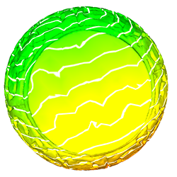
Figure 88.2 Isolines placed on a mesh without iDT remeshing
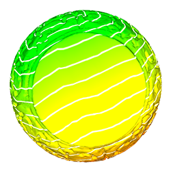
Figure 88.3 Isolines placed on a mesh with iDT remeshing
Performance
The time complexity of the algorithm is determined primarily by the choice of linear solver. In the current implementation, Cholesky prefactorization is roughly \(O(N^{1.5})\) and computation of distances is roughly \(O(N)\), where \( N\) is the number of vertices in the triangulation. The algorithm uses two \( N \times N\) matrices, both with the same pattern of non-zeros (in average 7 non-zeros per row/column). The cost of computation is independent of the size of the source set. Primitive operations include sparse numerical linear algebra (in double precision), and basic arithmetic operations (including square roots).
We perform the benchmark on an Intel Core i7-7700HQ, 2.8HGz, and compiled with Visual Studio 2013.
| Number of triangles | Initialization iDT (sec) | Distance computation iDT (sec) | Initialization Direct (sec) | Distance computation Direct (sec) |
|---|---|---|---|---|
| 30,000 | 0.18 | 0.02 | 0.12 | 0.01 |
| 200,000 | 1.82 | 1.31 | 1.32 | 0.11 |
| 500,000 | 10.45 | 0.75 | 8.07 | 0.55 |
| 1,800,000 | 38.91 | 2.24 | 35.68 | 1.1 |
Implementation History
This package was developed by Christina Vaz, Keenan Crane and Andreas Fabri as a project of the Google Summer of Code 2018.